A friend works in airborne LiDAR. The industry standard for the first step of every project — sorting the ground returns from the trees, buildings, cars, and noise — is a Bentley tool called TerraScan. It runs about ten grand a seat per year, lives inside MicroStation, and is Windows-only. Everything downstream of it (terrain models, contours, volumes, flood maps) depends on getting that one step right.
I had never opened a LAS file in my life. I spent yesterday evening with Claude Code and a Rust project folder.
This morning I had a working classifier.
0s
seconds end-to-end
0M
million points (Autzen)
0ft
ft RMSE vs pro
0
tests green
The job
Airborne LiDAR is a plane or drone firing a laser straight down a few hundred thousand times a second. Every pulse comes back as one or more 3D points — (x, y, z, intensity, return_number, ...). A normal survey is tens of millions to billions of these.
Before any of those points are useful, you have to label which ones are bare earth. That’s “ground classification.” The output is a new LAS file where the classification byte is set to 2 for ground points and left alone for everything else. Then you feed only the ground points into a gridder to make a DTM (digital terrain model), and the contours and volumes downstream all work.
TerraScan’s classic algorithm for this is Progressive TIN Densification (Axelsson 2000). You drop a coarse grid over the scene, take the lowest point in each cell as a ground seed, build a Delaunay TIN through the seeds, then iteratively add any point whose angle and distance to the nearest TIN facet are under some threshold. Repeat until no new points get added. The TIN is your ground surface.
The paper is six pages. The pseudocode is about a page. There is no good reason this needs to cost $10K/year and live inside MicroStation.
What I built
A Rust CLI called openscan. One self-contained binary. No PDAL, no GDAL, no Python, no system dependencies. It reads LAS 1.0–1.4 and LAZ (compressed LAS), classifies ground, and writes a new LAS/LAZ out with every other attribute and the coordinate reference system preserved untouched.
Two algorithms: Axelsson PTD (the TerraScan one) and Zhang’s Cloth Simulation Filter, ported faithfully from the reference mechanics — verlet gravity integration, structural/shear/bend springs, rigidness tables, post-constraint collision handling.
It tiles the cloud, fans the tiles across cores with rayon, and stitches the results with buffer halos so points near tile edges aren’t misclassified. It has an ISPRS-standard evaluator (Type I / Type II / total error / Cohen’s kappa) and a synthetic-scene generator so you can test against exact ground truth. DTM export drops a raster straight into QGIS plus a hillshade PNG.
Thirteen tests cover the math, both classifiers, outlier poisoning, tiled-vs-single-shot parity, DTM accuracy vs an analytic surface, and LAS/LAZ round-trip fidelity.
What it actually does
The hard part of PTD is the Delaunay TIN. In Rust, spade does the heavy lifting — a hierarchical Delaunay triangulation with point-location hints, which keeps the per-iteration cost bounded as the TIN grows. That part is just plumbing.
The interesting part is the parameter discipline. The whole algorithm hinges on six numbers, and if you get them wrong the classifier either keeps the trees or strips the ground:
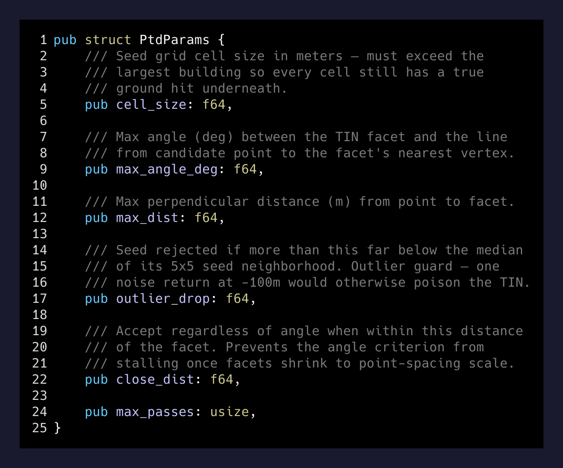
cell_size has to exceed the largest building footprint in the scene so every cell still contains at least one true ground hit underneath. outlier_drop is the median-based guard so a single noise return at -100m can’t poison the entire TIN. close_dist is a small but critical escape valve — once the TIN densifies down to point-spacing scale, the angle criterion stalls out, so any point closer than 20 cm to the facet gets accepted regardless of angle.
I didn’t know any of that going in. The model walked me through Axelsson’s original paper, the CSF reference implementation, and the failure modes the literature has documented over twenty-five years of follow-up work. Then it wrote the code.
The numbers
On a 1 km² synthetic scene with 2.06M points and exact ground truth (deterministic terrain + 40 buildings + 400 trees + 25 low outliers thrown in to try to poison the seed grid):
| Feature | Method | Type I | Type II | Total error | Kappa | Throughput |
|---|---|---|---|---|---|---|
| PTD (Axelsson) | 0.18% | 0.08% | 0.18% | 0.973 | 1.75M pts/s | |
| CSF (Zhang) | 0.17% | 0.94% | 0.28% | 0.957 | 3.59M pts/s |
Synthetic 1 km² benchmark with exact labeled truth.
For reference, ISPRS benchmark papers consider a kappa above 0.9 to be excellent. 0.97 is past the noise floor — most of the remaining “errors” are points whose true label is genuinely ambiguous (the bottom of a tree trunk, the edge of a roof gutter sitting on the ground).
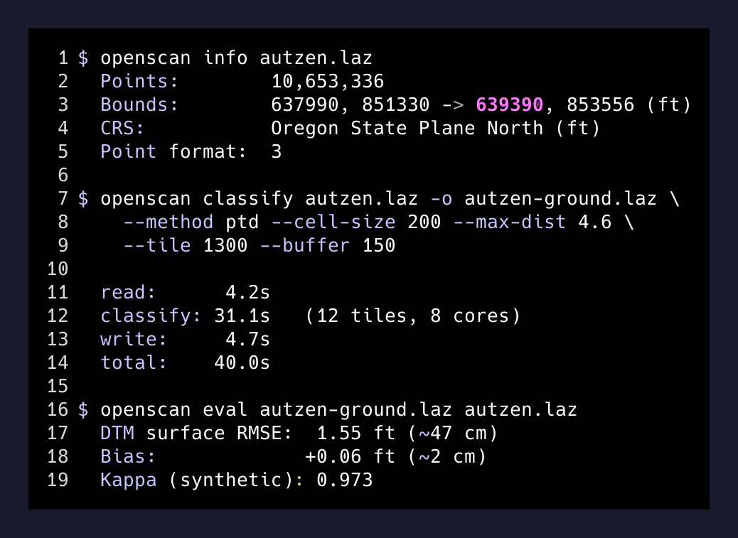
Then I ran it against real data — the Autzen Stadium benchmark, a publicly available 10.65M-point cloud from Eugene, Oregon, that’s been professionally classified by a working LiDAR contractor:
$ time ./target/release/openscan classify autzen.laz -o autzen-ground.laz \
    --method ptd --cell-size 200 --max-dist 4.6 --tile 1300 --buffer 150

read:      4.2s
classify:  31.1s
write:     4.7s
total:     40.0s

$ ./target/release/openscan eval autzen-ground.laz autzen.laz
DTM surface RMSE vs reference: 1.55 ft (~47 cm)
bias: +0.06 ft (~2 cm)
47 cm RMSE on a real-world dataset against a professional classification, in 40 seconds, on a desktop CPU.
The bare-earth hillshade it produces is, honestly, just pretty. Stadium berm resolved. River channel resolved. Road network resolved. Every tree and building stripped. No manual cleanup.
What I actually did versus what the model did
This is the part I want to be honest about.
The model wrote essentially all of the code. I wrote zero lines of Rust during the build. What I did was: pick the problem, set the scope (M0/M1 — single-machine, LAS in / LAS out, two algorithms, ISPRS evaluator, no viewer yet), and read every commit before accepting it.
What “reading every commit” means in practice: I checked that the seed-grid logic actually did what the paper said. I checked that the spring constants in the CSF port matched Zhang’s reference implementation. When the first synthetic eval came back with a suspiciously good kappa, I made it regenerate the scene with adversarial outliers and re-run. When the Autzen run took 90 seconds the first time, I asked where the time was going and we moved the per-tile triangulation behind a rayon parallel iterator.
That I now know LiDAR. I do not. I know enough about this one algorithm to recognize when the output is wrong, which is a much lower bar than knowing the field.
— What I'm not claiming
There is a real version of this where someone vibe-codes a “LiDAR classifier,” it produces something that looks plausible on the input that was used to develop it, and it silently mislabels half the ground on a real dataset. The thing that prevented that here was the ISPRS evaluator, the synthetic scene with known truth, and the real-world benchmark against a professional classification — all built before the classifier did its first real run. If you’re not going to test against ground truth, you’re not building a classifier. You’re producing a confident-looking lie.
Why this matters
Two things, mostly.
One: ground classification is the wedge for a whole product. Every downstream LiDAR workflow — DTM, contours, volumes, flood modeling, hydrology, hillshade — depends on it. If you ship a fast, correct, open classifier with an integrated inspect-and-fix loop (CloudCompare and LAStools both lack this), you’ve cracked open the most expensive node in a $10K/year Windows-only stack. The next milestones in the project are a viewer with manual edit, out-of-core streaming so you can chew through billion-point clouds without melting RAM, and COPC support. Each one is another vertical slice cut out of the incumbent.
Two: the time-cost of “I should learn this domain” has collapsed. A decade ago, the path to writing a classifier like this looked like a graduate seminar plus six months. Yesterday it looked like an evening with a model that had read every relevant paper and could turn out idiomatic Rust against las-rs and spade without me checking syntax. The bottleneck is no longer typing or research. It’s having a good test against ground truth, and the taste to recognize when the output is wrong.
That second one is the durable skill. The classifier is the byproduct.